目录
- 一、shapely模块
- 1、shapely
- 2、point→Point类
- 3、导入所需模块
- 4、Point
- (1)、创建point,主要有以下三种方法
- (2)、point常用属性
- (3)、point常用方法,计算距离
- 5、LineString
- 6、LineRing:(是一个封闭图形)
- 7、Polygon:(多边形)
- 8、几何对象的关系:内部、边界与外部
- 9、point、LineRing、LineString与numpy中的array互相转换
- 二、geopandas模块
- 1、导入模块
- 2、geohash_encode编码函数
一、shapely模块
1、shapely
shapely是python中开源的针对空间几何进行处理的模块,支持点、线、面等基本几何对象类型以及相关空间操作。
2、point→Point类
curve→LineString和LinearRing类;
surface→Polygon类
集合方法分别对应MultiPoint、MultiLineString、MultiPolygon
3、导入所需模块
# 导入所需模块
from shapely import geometry as geo
from shapely import wkt
from shapely import ops
import numpy as np
from shapely.geometry.polygon import LinearRing
from shapely.geometry import Polygon
from shapely.geometry import asPoint, asLineString, asMultiPoint, asPolygon
4、Point
(1)、创建point,主要有以下三种方法
# 创建point
pt1 = geo.Point([0,0])
coord = np.array([0,1])
pt2 = geo.Point(coord)
pt3 = wkt.loads("POINT(1 1)")
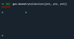
geo.GeometryCollection([pt1, pt2, pt3]) #批量可视化
最终三个点的结果如下所示:
(2)、point常用属性
# point常用属性
print(pt1.x) #pt1的x坐标
print(pt1.y)#pt1的y坐标
print(list(pt1.coords))
print(np.array(pt1))
输出结果如下:
0.0
0.0
[(0.0, 0.0)]
[0. 0.]
(3)、point常用方法,计算距离
# point计算距离
d = pt2.distance(pt1) #计算pt1与pt2的距离, d =1.0
5、LineString
创建LineString主要有以下三种方法:
# LineString的创建
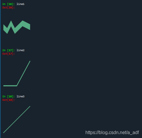
line1 = geo.LineString([(0,0),(1,-0.1),(2,0.1),(3,-0.1),(5,0.1),(7,0)])
arr = np.array([(2, 2), (3, 2), (4, 3)])
line2 = geo.LineString(arr)
line3 = wkt.loads("LineString(-2 -2,4 4)")
line1, line2, line3对应的直线如下所示
LineString常用方法:
print(line2.length) #计算线段长度:2.414213562373095
print(list(line2.coords)) #线段中点的坐标:[(2.0, 2.0), (3.0, 2.0), (4.0, 3.0)]
print(np.array(line2)) #将点坐标转成numpy.array形式[[2. 2.],[3. 2.],[4. 3.]]
print(line2.bounds)#坐标范围:(2.0, 2.0, 4.0, 3.0)
center = line2.centroid #几何中心:
geo.GeometryCollection([line2, center])
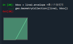
bbox = line2.envelope #最小外接矩形
geo.GeometryCollection([line2, bbox])
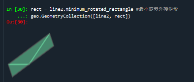
rect = line2.minimum_rotated_rectangle #最小旋转外接矩形
geo.GeometryCollection([line2, rect])
line2几何中心:

line2的最小外接矩形:
line2的最小旋转外接矩形:
#常用方法
d1 = line1.distance(line2) #线线距离: 1.9
d2 = line1.distance(geo.Point([-1, 0])) #点线距离:1.0
d3 = line1.hausdorff_distance(line2) #最大最小距离:4.242640687119285
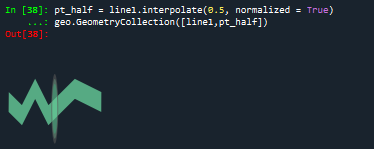
#插值
pt_half = line1.interpolate(0.5, normalized = True)
geo.GeometryCollection([line1,pt_half])
#投影
ratio = line1.project(pt_half, normalized = True)
print(ratio)#project()方法是和interpolate方法互逆的:0.5
插值:
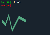
DouglasPucker算法:道格拉斯-普克算法:是将曲线近似表示为一系列点,并减少点的数量的一种算法。
#DouglasPucker算法
line1 = geo.LineString([(0, 0), (1, -0.2), (2, 0.3), (3, -0.5), (5, 0.2), (7,0)])
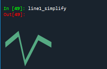
line1_simplify = line1.simplify(0.4, preserve_topology=False)
print(line1)#LINESTRING (0 0, 1 -0.1, 2 0.1, 3 -0.1, 5 0.1, 7 0)
print(line1_simplify)#LINESTRING (0 0, 2 0.3, 3 -0.5, 5 0.2, 7 0)
buffer_with_circle = line1.buffer(0.2) #端点按照半圆扩展
geo.GeometryCollection([line1,buffer_with_circle])
道格拉斯-普克算法化简后的结果
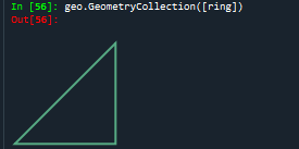
6、LineRing:(是一个封闭图形)
#LinearRing是一个封闭图形
ring = LinearRing([(0, 0), (1, 1), (1, 0)])
print(ring.length)#相比于刚才的LineString的代码示例,其长度现在是3.41,是因为其序列是闭合的
print(ring.area):结果为0
geo.GeometryCollection([ring])
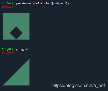
7、Polygon:(多边形)
polygonl = Polygon([(0, 0), (1, 1), (1, 0)])
ext = [(0, 0), (0, 2), (2, 2), (2, 0), (0, 0)]
int1 = [(1, 0), (0.5, 0.5), (1, 1), (1.5, 0.5), (1, 0)]
polygon2 = Polygon(ext, [int1])
print(polygonl.area)#几何对象的面积:0.5
print(polygonl.length)#几何对象的周长:3.414213562373095
print(polygon2.area)#其面积是ext的面积减去int的面积:3.5
print(polygon2.length)#其长度是ext的长度加上int的长度:10.82842712474619
print(np.array(polygon2.exterior)) #外围坐标点:
#[[0. 0.]
 #[0. 2.]
 #[2. 2.]
 #[2. 0.]
# [0. 0.]]
geo.GeometryCollection([polygon2])
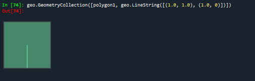
8、几何对象的关系:内部、边界与外部
#obj.contains(other) == other.within(obj)
coords = [(0, 0), (1, 1)]
print(geo.LineString(coords).contains(geo.Point(0.5, 0.5)))#包含:True

print(geo.LineString(coords).contains(geo.Point(1, 1)))#False
polygon1 = Polygon([(0, 0), (0, 2), (2, 2), (2, 0), (0, 0)])
print(polygon1.contains(geo.LineString([(1.0, 1.0), (1.0, 0)])))#面与线关系:True
#contains方法也可以扩展到面与线的关系以及面与面的关系
geo.GeometryCollection([polygon1, geo.LineString([(1.0, 1.0), (1.0, 0)])])
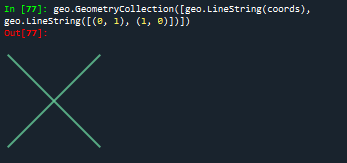
#obj.crosses(other):相交与否
print(geo.LineString(coords).crosses(geo.LineString([(0, 1), (1, 0)])))#:True
geo.GeometryCollection([geo.LineString(coords), geo.LineString([(0, 1), (1, 0)])])
#obj.disjoint(other):均不相交返回True
print(geo.Point(0, 0).disjoint(geo.Point(1, 1)))
#object.intersects(other)如果该几何对象与另一个几何对象只要相交则返回True。
print(geo.LineString(coords).intersects(geo.LineString([(0, 1), (1, 0)])))#True
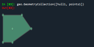
#object.convex_hull返回包含对象中所有点的最小凸多边形(凸包)
points1 = geo.MultiPoint([(0, 0), (1, 1), (0, 2), (2, 2), (3, 1), (1, 0)])
hull1 = points1.convex_hull
geo.GeometryCollection([hull1, points1])
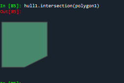
#object.intersection  返回对象与对象之间的交集
polygon1 = Polygon([(0, 0), (0, 2), (2, 2), (2, 0), (0, 0)])
hull1.intersection(polygon1)
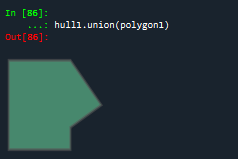
#返回对象与对象之间的并集
hull1.union(polygon1)
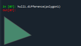
#面面补集
hull1.difference(polygon1)
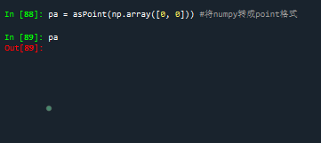
9、point、LineRing、LineString与numpy中的array互相转换
pa = asPoint(np.array([0, 0])) #将numpy转成point格式
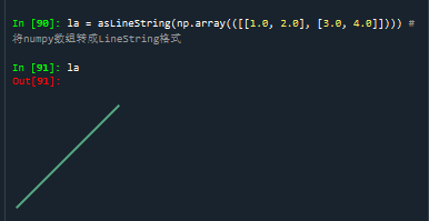
 #将numpy数组转成LineString格式
la = asLineString(np.array(([[1.0, 2.0], [3.0, 4.0]])))
#将numpy数组转成multipoint集合
ma = asMultiPoint(np.array([[1.1, 2.2], [3.3, 4.4], [5.5, 6.6]]))
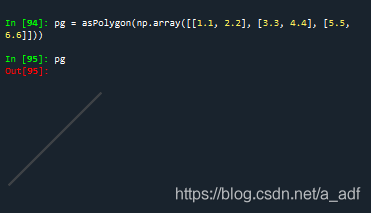
#将numpy转成多边形
pg = asPolygon(np.array([[1.1, 2.2], [3.3, 4.4], [5.5, 6.6]]))
二、geopandas模块
geopandas拓展了pandas,共有两种数据类型:GeoSeries、GeoDataFrame
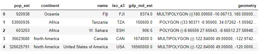
下述是利用geopandas库绘制世界地图:
import pandas as pd
import geopandas
import matplotlib.pyplot as plt
world = geopandas.read_file(geopandas.datasets.get_path('naturalearth_lowres')) #read_file方法可以读取shape文件
world.plot()
plt.show()

#根据每一个polygon的pop_est不同,便可以用python绘制图表显示不同国家的人数
fig, ax = plt.subplots(figsize = (9, 6), dpi = 100)
world.plot('pop_est', ax = ax, legend =True)
plt.show()

python对海洋数据进行预处理操作(这里我发现,tqdm模块可以显示进度条,感觉很高端,像下面这样)

1、导入模块
```python
import pandas as pd
import geopandas as gpd
from pyproj import Proj #左边转换
from keplergl import KeplerGl
from tqdm import tqdm
import os
import matplotlib.pyplot as plt
from matplotlib.lines import Line2D
import shapely
import numpy as np
from datetime import datetime
import warnings
warnings.filterwarnings('ignore')
plt.rcParams['font.sans-serif'] = ['SimSun'] #指定默认字体为新宋体
plt.rcParams['axes.unicode_minus'] = False
DataFrame获取数据,坐标转换,计算距离
#获取文件夹中的数据
def get_data(file_path, model):
assert model in ['train', 'test'], '{} Not Support this type of file'.format(model)
paths = os.listdir(file_path)
tmp = []
for t in tqdm(range(len(paths))):
p = paths[t]
with open('{}/{}'.format(file_path, p), encoding = 'utf-8') as f:
next(f) #读取下一行
for line in f.readlines():
tmp.append(line.strip().split(','))
tmp_df = pd.DataFrame(tmp)
if model == 'train':
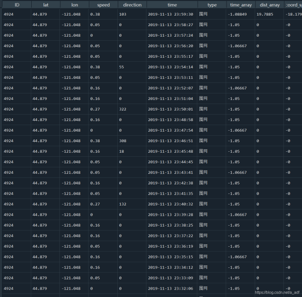
tmp_df.columns = ['ID', 'lat', 'lon', 'speed', 'direction', 'time', 'type']
else:
tmp_df['type'] = 'unknown'
tmp_df.columns = ['ID', 'lat', 'lon', 'speed', 'direction', 'time', 'type']
tmp_df['lat'] = tmp_df['lat'].astype(float)
tmp_df['lon'] = tmp_df['lon'].astype(float)
tmp_df['speed'] = tmp_df['speed'].astype(float)
tmp_df['direction'] = tmp_df['direction'].astype(int)
return tmp_df
file_path = r"C:\Users\李\Desktop\datawheal\数据\hy_round1_train_20200102"
model = 'train'
#平面坐标转经纬度
def transform_xy2lonlat(df):
x = df['lat'].values
y = df['lon'].values
p = Proj('+proj=lcc +lat_1=33.88333333333333 +lat_2=32.78333333333333 +lat_0=32.16666666666666 +lon_0=-116.25 +x_0=2000000.0001016 +y_0=500000.0001016001 +datum=NAD83 +units=us-ft +no_defs ')
df['lon'], df['lat'] = p(y, x, inverse = True)
return df
#修改数据的时间格式
def reformat_strtime(time_str = None, START_YEAR = '2019'):
time_str_split = time_str.split(" ") #以空格为分隔符
time_str_reformat = START_YEAR + '-' + time_str_split[0][:2] + "-" + time_str_split[0][2:4]
time_str_reformat = time_str_reformat + " " + time_str_split[1]
return time_str_reformat
#计算两个点的距离
def haversine_np(lon1, lat1, lon2, lat2):
lon1, lat1, lon2, lat2 = map(np.radians, [lon1, lat1, lon2, lat2])
dlon = lon2 - lon1
dlat = lat2 - lat1
a = np.sin(dlat/2.0)**2 + np.cos(lat1) * np.cos(lat2) * np.sin(dlon/2.0)**2
c = 2 * np.arcsin(np.sqrt(a))
km = 6367 * c
return km * 1000
利用3-sigma算法对异常值进行处理,速度与时间
#计算时间的差值
def compute_traj_diff_time_distance(traj = None):
    #计算时间的差值
    time_diff_array = (traj['time'].iloc[1:].reset_index(drop = True) - traj['time'].iloc[:-1].reset_index(drop = True)).dt.total_seconds() / 60
    #计算坐标之间的距离
    dist_diff_array = haversine_np(traj['lon'].values[1:],
                                   traj['lat'].values[1:],
                                   traj['lon'].values[:-1],
                                   traj['lat'].values[:-1])
    #填充第一个值
    time_diff_array = [time_diff_array.mean()] + time_diff_array.tolist()
    dist_diff_array = [dist_diff_array.mean()] + dist_diff_array.tolist()
    traj.loc[list(traj.index), 'time_array'] = time_diff_array
    traj.loc[list(traj.index), 'dist_array'] = dist_diff_array
    return traj
#对轨迹进行异常点的剔除
def assign_traj_anomaly_points_nan(traj = None, speed_maximum = 23,time_interval_maximum = 200, coord_speed_maximum = 700):
    #将traj中的异常点分配给np.nan
    def thigma_data(data_y, n):
        data_x = [i for i in range(len(data_y))]
        ymean = np.mean(data_y)
        ystd = np.std(data_y)
        threshold1 = ymean - n * ystd
        threshold2 = ymean + n * ystd
        judge = []
        for data in data_y:
            if data < threshold1 or data > threshold2:
                judge.append(True)
            else:
                judge.append(False)
        return judge
    #异常速度修改
    is_speed_anomaly = (traj['speed'] > speed_maximum) | (traj['speed'] < 0)
    traj['speed'][is_speed_anomaly] = np.nan
    #根据距离和时间计算速度
    is_anomaly = np.array([False] * len(traj))
    traj['coord_speed'] = traj['dist_array'] / traj['time_array']
    #根据3-sigma算法对速度剔除以及较大的时间间隔点
    is_anomaly_tmp = pd.Series(thigma_data(traj['time_array'], 3)) | pd.Series(thigma_data(traj['coord_speed'], 3))
    is_anomaly = is_anomaly | is_anomaly_tmp
    is_anomaly.index = traj.index
    #轨迹点的3-sigma异常处理
    traj = traj[~is_anomaly].reset_index(drop = True)
    is_anomaly = np.array([False]*len(traj))
    if len(traj) != 0:
        lon_std, lon_mean = traj['lon'].std(), traj['lon'].mean()
        lat_std, lat_mean = traj['lat'].std(), traj['lat'].mean()
        lon_low, lon_high = lon_mean - 3* lon_std, lon_mean + 3 * lon_std
        lat_low, lat_high = lat_mean - 3 * lat_std, lat_mean + 3 * lat_std
        is_anomaly = is_anomaly | (traj['lon'] > lon_high) | ((traj['lon'] < lon_low))
        is_anomaly = is_anomaly | (traj["lat"] > lat_high) | ((traj["lat"] < lat_low))
        traj = traj[~is_anomaly].reset_index(drop = True)
    return traj, [len(is_speed_anomaly) - len(traj)]

file_path = r"C:\Users\李\Desktop\datawheal\数据\hy_round1_train_20200102"
model = 'train'
df = get_data(file_path, model)
#转换时间格式
df = transform_xy2lonlat(df)
df['time'] = df['time'].apply(reformat_strtime)
df['time'] = df['time'].apply(lambda x: datetime.strptime(x,'%Y-%m-%d %H:%M:%S'))
#对轨迹的异常点进行剔除,对缺失值进行线性插值处理
ID_list = list(pd.DataFrame(df['ID'].value_counts()).index)
DF_NEW = []
Anomaly_count = []
for ID in tqdm(ID_list):
    # print(ID)
    df_id = compute_traj_diff_time_distance(df[df['ID'] == ID])
    df_new, count = assign_traj_anomaly_points_nan(df_id)
    df_new['speed'] = df_new['speed'].interpolate(method = 'linear', axis = 0)
    df_new = df_new.fillna(method = 'bfill') #用前一个非缺失值取填充该缺失值
    df_new = df_new.fillna(method = 'ffill')#用后一个非缺失值取填充该缺失值
    df_new['speed'] = df_new['speed'].clip(0, 23) #clip()函数将其限定在0,23
    Anomaly_count.append(count) #统计每个id异常点的数量有多少
    DF_NEW.append(df_new)
DF = pd.concat(DF_NEW)
处理后的DF
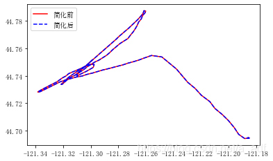
利用Geopandas中的Simplify进行轨迹简化和压缩
#道格拉斯-普克,由该案例可以看出针对相同的ID轨迹,可以先用geopandas将其进行简化和数据压缩
line = shapely.geometry.LineString(np.array(df[df['ID'] == '11'][['lon', 'lat']]))
ax = gpd.GeoSeries([line]).plot(color = 'red')
ax = gpd.GeoSeries([line]).simplify(tolerance = 0.000000001).plot(color = 'blue', ax = ax, linestyle = '--')
LegendElement = [Line2D([], [], color = 'red', label = '简化前'),
                 Line2D([], [], color = 'blue', linestyle = '--', label = '简化后')]
#将制作好的图例影响对象列表导入legend()中
ax.legend(handles = LegendElement, loc = 'upper left', fontsize = 10)
print('化简前数据长度:' + str(len(np.array(gpd.GeoSeries([line])[0]))))
print('化简后数据长度' + str(len(np.array(gpd.GeoSeries([line]).simplify(tolerance = 0.000000001)[0]))))
#定义数据简化函数,通过shapely库将经纬度转换成LineString格式,然后通过GeoSeries数据结构中利用simplify进行简化,再将所有数据放入GeoDataFrame
def simplify_dataframe(df):
    line_list = []
    for i in tqdm(dict(list(df.groupby('ID')))):
        line_dict = {}
        lat_lon = dict(list(df.groupby('ID')))[i][['lon', 'lat']]
        line = shapely.geometry.LineString(np.array(lat_lon))
        line_dict['ID'] = dict(list(df.groupby('ID')))[i].iloc[0]['ID']
        line_dict['type'] = dict(list(df.groupby('ID')))[i].iloc[0]['type']
        line_dict['geometry'] = gpd.GeoSeries([line]).simplify(tolerance = 0.000000001)[0]
        line_list.append(line_dict)
    return gpd.GeoDataframe(line_list)
化简前数据长度:377
化简后数据长度156
这块的df_gpd_change没有读出来,后续再发
df_gpd_change=pd.read_pickle(r"C:\Users\李\Desktop\datawheal\数据\df_gpd_change.pkl")
map1=KeplerGl(height=800)#zoom_start与这个height类似,表示地图的缩放程度
map1.add_data(data=df_gpd_change,name='data')
#当运行该代码后,下面会有一个kepler.gl使用说明的链接,可以根据该链接进行学习参
GeoHash编码:利用二分法不断缩小经纬度区间,经度区间二分为[-180, 0]和[0,180],纬度区间二分为[-90,0]和[0,90],偶数位放经度,奇数位放纬度交叉,将二进制数每五位转化为十进制,在对应编码表进行32位编码
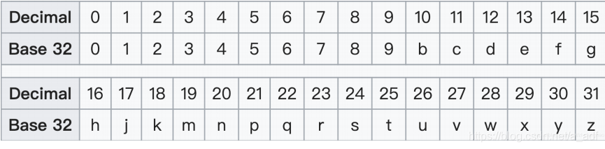
2、geohash_encode编码函数
def geohash_encode(latitude, longitude, precision = 12):
    lat_interval, lon_interval = (-90.0, 90.0), (-180, 180)
    base32 = '0123456789bcdefghjkmnpqrstuvwxyz'
    geohash = []
    bits = [16, 8, 4, 2, 1]
    bit = 0
    ch = 0
    even = True
    while len(geohash) < precision:
        if even:
            mid = (lon_interval[0] + lon_interval[1]) / 2
            if longitude > mid:
                ch |= bits[bit]
                lon_interval = (mid, lon_interval[1])
            else:
                lon_interval = (lon_interval[0], mid)
        else:
            mid = (lat_interval[0] + lat_interval[1]) / 2
            if latitude > mid:
                ch |= bits[bit]
                lat_interval = (mid, lat_interval[1])
            else:
                lat_interval = (lat_interval[0], mid)
        even = not even
        if bit < 4:
            bit += 1
        else:
            geohash += base32[ch]
            bit = 0
            ch = 0
    return ''.join(geohash)
jsjbwy